
Georgia Huang




| Picture | Part Number | Manufacturer | Stock | Action |
|---|---|---|---|---|
 | LSM6DSV16XTR | STMicroelectronics | 5,880 | |
 | LSM6DSV32XTR | STMicroelectronics | 6,690 | |
 | LSM6DSV16BXTR | STMicroelectronics | 7,950 | |
 | ISM330DHCXTR | STMicroelectronics | 6,520 | |
 | LSM6DSOXTR | STMicroelectronics | 4,630 |
The available sources do not establish that a particular robot or flight controller is certified or in production with this device. Its acceleration, angular-rate and embedded processing capabilities make it a candidate to evaluate when they fit the task. Qualification remains a system-level decision involving mounting, local temperature, timing, software and the required machine behavior. Industrial-robot installation statistics describe an application market; they do not prove adoption, shipments or current demand for this exact ordering code.
The datasheet requires the gyroscope OIS chain to be disabled when the ±4000 dps UI gyroscope range is selected. Resolve that restriction before choosing a simultaneous-channel configuration. Also avoid applying the typical 2.8 mdps/√Hz noise-density statement unqualified at the widest range: the datasheet's stated range independence extends only through ±2000 dps. Evaluate the range from expected peaks and clipping, then recheck scale factors, filtering and downstream thresholds under the selected configuration.
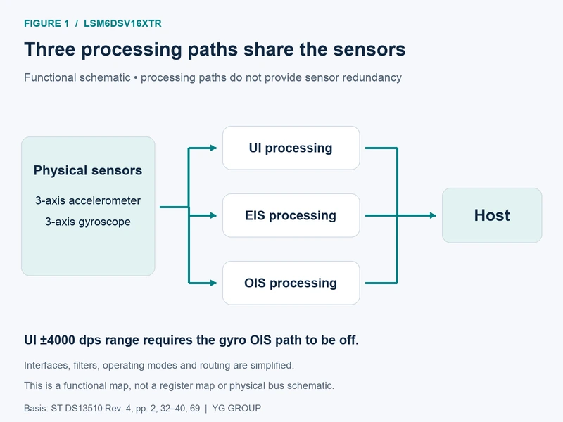
No. UI, EIS and OIS are processing paths that share the physical acceleration and angular-rate sensing elements. They can serve different data consumers, subject to supported configuration combinations, but they should not be counted as independent IMUs in a reliability argument. If the robot needs redundant sensing, define that requirement separately. For a multi-consumer design, document each stream's range, filtering, interface and timing needs, then verify that the chosen combination delivers them together.
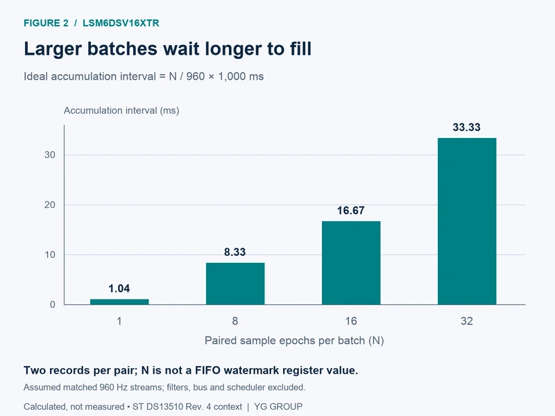
Distinguish 1.5 KB of raw storage from the advertised effective capacity of up to 4.5 KB with compression. A simple uncompressed acceleration-plus-gyro transport estimate uses two seven-byte tagged records per sampling epoch, before timestamps, other outputs and bus overhead. Larger batches reduce transaction frequency but age the oldest data. At 960 epochs per second, collecting 32 pairs spans about 33.33 milliseconds ideally; this is a conceptual fill interval, not a watermark register value or total measured latency.
No. The low-power fusion outputs can help an application, but six-axis inertial sensing does not supply an independent absolute heading reference. Bias, motion conditions and timing still affect how the data should be used. Combine the observations with encoders, cameras or other references according to the estimator's requirements. Check the output rates as well: embedded fusion and classification rates differ from the fastest raw sensor rates, so a new raw sample does not necessarily imply a new embedded result.
Compare LSM6DSV32XTR for acceleration ranges extending to ±32 g, LSM6DSV16BXTR for motion with audio-related capabilities, ISM330DHCXTR when industrial positioning and operation up to +105°C matter, and LSM6DSOXTR when a gyroscope range through ±2000 dps is sufficient. These are distinct base sensors with different tradeoffs. Their relationship does not establish drop-in compatibility. Recheck electrical interfaces, filtering, register behavior, package details and the complete mounted-system performance before approving a change.
By Georgia Huang
STMicroelectronics' LSM6DSV16XTR combines three-axis acceleration and angular-rate sensing with configurable processing and embedded motion functions. It is a candidate to evaluate for robot motion feedback, vibration observation and local event detection when its range, temperature limits and timing behavior fit the machine. Robot-market growth provides a reason to examine those needs; it does not establish adoption of this component. Selection should follow the robot's actual movement and data path.
Robot installations create demand for many kinds of components, but the relationship to any particular IMU is indirect. The International Federation of Robotics reported 542,000 industrial robots installed worldwide in 2024 in its September 2025 World Robotics release. A separate June 18, 2026 announcement put preliminary US installations in 2025 at 38,000, up 11% year over year. These figures describe different geographical and reporting periods; the US result is preliminary. IFR global report, IFR US update.
Neither figure identifies the sensors fitted to those robots. A large stationary arm, a small mobile platform and a camera-equipped inspection device have different motion-sensing requirements. Some rely heavily on encoders and external references; others need inertial measurements to bridge gaps between those observations. Unit growth cannot be converted into LSM6DSV16XTR sales, a design-win claim or a shortage forecast without additional evidence.
For an engineering team, the useful implication is narrower: define where motion data improves the machine's behavior. A sensor might help detect an abnormal chassis impact, estimate short-term rotation or identify a vibration state. Each task imposes a different balance of bandwidth, dynamic range, latency and false alarms. A low-power feature is valuable only if it preserves the information required by that task.
Treat the device as an evaluation candidate whose suitability must be established on the robot, not as a robot-qualified component based on market growth. ST's published applications include motion tracking, indoor navigation and vibration monitoring, but those descriptions do not establish certification of a particular robot or flight controller. The board, software and machine-level validation remain part of the selection decision.
An IMU measures acceleration and angular rate at its mounting location. Those measurements need interpretation before they become velocity, attitude or a useful machine event. Gravity contributes to an accelerometer's reading, while a sensor placed away from a rotation center can see motion that differs from the motion of the chassis reference point. The location and coordinate convention belong in the system model.
A mobile robot moving across a threshold may produce a short acceleration peak that is unimportant to navigation but important to impact detection. A rotating joint may create a sustained angular rate with superimposed vibration. A camera payload may need a fast stabilization stream alongside a slower application stream. Begin by separating those tasks instead of asking one filtered output to satisfy every consumer.
Table 1. Translate a robot function into a measurable IMU requirement.
| Intended function | Motion information needed | Evaluation priority | Decision evidence |
|---|---|---|---|
| Chassis attitude support | Rotation and gravity-related observations | Bias, alignment and usable latency | Comparison with an independent reference |
| Impact or handling detection | Short transient acceleration | Clipping and event capture | Labeled impacts across mounting conditions |
| Vibration observation | Frequency content at the mounting point | Bandwidth, filtering and aliasing | Repeatable excitation and spectral comparison |
| Local motion-state classification | Features that distinguish operating states | False alarms and generalization | Held-out data from different runs and units |
| Camera-associated motion | Separate consumers with different timing needs | Channel compatibility and synchronization | Simultaneous-stream timing measurements |
Selecting the largest range and highest output rate does not necessarily produce the most useful stream. Wider range changes scale factor. Higher output rate increases transport and processing work. Stronger filtering suppresses unwanted components but can also delay useful information. The right setting follows the decision the robot needs to make.
Establish the sensor axes relative to the robot frame, including signs and the direction used for positive rotation. Check the convention with simple controlled movements before running a complicated route. A clean-looking plot can still be physically wrong if an axis is swapped or a coordinate transform is applied twice.
Mount the evaluation board firmly enough that its motion represents the intended measurement point. A loose cable, flexible carrier or unsupported board edge can introduce a local vibration mode. Moving the board to a more convenient location can also change the observation. Preserve photographs or mechanical coordinates in the engineering record so a later data collection can reproduce the setup.
Keep raw measurements and configuration information during early evaluation. A fused or classified output is convenient, but it can hide clipping, dropped samples or a filter configuration error. Raw data gives the team a way to investigate why a higher-level result changed. The storage cost is often worthwhile during the phase when the mounting and signal chain are still being selected.
The device provides selectable acceleration ranges from ±2 g to ±16 g and gyroscope ranges from ±125 dps to ±4000 dps. Those endpoints describe selectable measurement ranges, not accuracy over arbitrary motion. The supplied datasheet identifies the tape-and-reel ordering code as LSM6DSV16XTR and specifies an operating temperature range of −40 to +85°C. ST DS13510 Rev 4, pages 1 and 12–14.
Table 2. Useful specifications and the conditions that keep them meaningful.
| Parameter | Documented value | Condition or limitation | Selection consequence |
|---|---|---|---|
| Acceleration full scale | ±2, ±4, ±8 or ±16 g | Sensitivity changes with selected range | Check both expected peaks and required resolution |
| Gyroscope full scale | ±125 through ±4000 dps | ±4000 dps requires the gyroscope OIS chain disabled | Confirm simultaneous-channel requirements first |
| Gyroscope noise density | 2.8 mdps/√Hz typical | High-performance mode; stated range independence only through ±2000 dps | Do not carry this figure unqualified into the widest range |
| Accelerometer noise density | 60 µg/√Hz typical | High-performance mode with dual-channel acceleration disabled | Revisit the estimate if the channel configuration changes |
| Combined high-performance current | 0.65 mA typical | VDD 1.8 V and 25°C unless otherwise noted | Measure the complete board under its actual duty cycle |
| Operating temperature | −40 to +85°C | Device operating range | Compare with sensor-local temperature in the enclosure |
Noise and current figures in this table are typical values from the datasheet's stated conditions, not guaranteed maxima. Low current can help a battery-powered platform, while suitable noise performance can preserve a small motion signal. Neither replaces a measurement of the actual mounted system under its operating conditions.
At ±2 g, the nominal acceleration sensitivity is 0.061 mg per least significant bit; at ±16 g it is 0.488 mg per least significant bit. The wider range accommodates larger excursions but assigns a larger physical increment to each output count. Those scale factors do not mean the effective measurement resolution equals one count, because noise, offset and the complete signal chain also matter.
Begin with recorded or conservatively estimated motion peaks. Include normal maneuvers, startup, transport and credible impacts that the application is expected to measure. A shock-survival rating is a different specification: surviving an event does not mean measuring that event without saturation or preserving useful accuracy throughout it.
Use ±4000 dps only after confirming that the gyroscope OIS chain can be disabled. The datasheet explicitly attaches that restriction to the setting. A product that requires OIS simultaneously should resolve the channel requirement before relying on the maximum angular-rate range. This is a functional compatibility check, not a minor footnote to postpone until firmware integration.
During evaluation, log how often samples approach the full-scale limit and inspect the surrounding waveform. A flat-topped transient can hide the real peak and distort derived features. Increasing the range may solve clipping, but it also changes scale factors used by downstream code. Revalidate thresholds and calibration handling whenever a range changes.
The 0.65 mA combined high-performance figure is typical at 1.8 V and 25°C, under the datasheet's stated conditions. It is useful for an initial sensor budget. It is not the current of an evaluation board, host processor or complete robot. Regulators, interface activity, pull-ups and the host's wake time can dominate the benefit of a lower sensor-only current.
Measure the states that the product actually uses: continuous motion tracking, waiting for an event, processing a burst and returning to a lower-power state. Include the time needed to obtain valid data after a transition. A mode that saves current while waiting may provide little system benefit if it forces long host activity or misses the beginning of an event.
Temperature deserves a similar system-level treatment. Ambient room temperature may differ substantially from the temperature near a motor driver or inside a sealed housing. Test after thermal stabilization and during representative transitions. If the required local operating range exceeds the device's specified limits, select a more suitable candidate instead of treating a successful room-temperature demonstration as an exception to the specification.
The triple-channel architecture provides user-interface (UI), electronic image stabilization (EIS) and optical image stabilization (OIS) processing paths for different data consumers. It does not provide three independent accelerometers and three independent gyroscopes. The channels share the physical sensing elements, so they should not be counted as redundant sensors in a reliability argument. ST DS13510 Rev 4, pages 2 and 32–40.
For a robot with a camera, separate processing paths may help satisfy different filtering and timing needs. The benefit is strongest when those needs are explicit. List each consumer, its required signal, its acceptable delay and the interface through which it receives data. Then check whether the intended combination is supported before configuring every attractive feature at once.
A high output data rate tells the host how often new values can arrive. It does not mean every frequency below that rate passes unchanged. The gyroscope UI path's documented LPF2 cutoff is 342 Hz at a 960 Hz output rate, under the listed filter arrangement. Other filtering choices change the signal further. A useful design record names both the output rate and the active filter chain.
Filtering should follow the motion task. A navigation estimator may benefit from suppressing high-frequency chassis vibration, while a vibration diagnostic may need to retain that same content. If both functions use one stream, a filter that improves one may damage the other. Separate channels or separate processing can help, but only within the device's supported combinations.
The optional UI gyroscope LPF1 is available under specific conditions and is unavailable when OIS or EIS is enabled. Do not transfer a filter setting from a single-channel demonstration into a simultaneous-channel design without rechecking it. The waveform and timing need to be compared again after the channel arrangement changes.
A digital filter also cannot justify ignoring all out-of-band mechanical excitation. Identify the frequencies produced by motors, gears and structural resonances, then verify the chosen sampling and filtering configuration with representative excitation. A low-frequency artifact in the recorded data may originate from a much faster physical vibration. Testing a stationary board on a quiet desk will not reveal that risk.
The internal timestamp is a 32-bit value with a typical 21.75 microsecond increment. That describes timestamp resolution; it is not a guarantee that a sample is aligned to the robot controller's clock within that interval. Clock differences, reading order and software scheduling still affect how measurements are placed on the system timeline. ST DS13510 Rev 4, pages 85 and 90.
Measure or establish the relationship between sensor time and host time. Preserve sample order across FIFO reads and handle wraparound deliberately. If the host timestamps a batch only when its interrupt handler runs, every sample in that batch must not be treated as though it was acquired at that instant. Older samples need their proper temporal position.
For systems that combine camera, encoder and inertial data, timing errors can look like calibration errors. A turn observed late by one stream may produce a disagreement that persists even after adjusting scale factors. Verify timing before spending extensive effort tuning an estimator around inconsistent observations.
The FIFO supports 1.5 KB of raw data storage, with up to 4.5 KB effective capacity when compression is used. Do not budget every stream as though 4.5 KB of uncompressed storage were available. Compression behavior and the enabled data types matter. The host must also understand the tagged records and the selected FIFO mode. ST DS13510 Rev 4, pages 44–46.
An uncompressed accelerometer or gyroscope record contains a one-byte tag and six bytes of data. For a simple transport estimate with both streams at the same rate, two records require fourteen bytes per sampling epoch. This estimates bytes the host must retrieve for those two streams; it excludes timestamp records, other enabled outputs, transaction overhead and bus signaling.
Table 3. Calculated uncompressed record traffic for equal-rate acceleration and gyroscope streams.
| Rate of each stream | Records per second across both streams | Record bytes per second | What the estimate excludes |
|---|---|---|---|
| 120 Hz | 240 | 1,680 | Timestamp and other records; bus overhead |
| 240 Hz | 480 | 3,360 | Timestamp and other records; bus overhead |
| 480 Hz | 960 | 6,720 | Timestamp and other records; bus overhead |
| 960 Hz | 1,920 | 13,440 | Timestamp and other records; bus overhead |
| 1,920 Hz | 3,840 | 26,880 | Timestamp and other records; bus overhead |
The arithmetic is fourteen bytes times the selected rate. It does not establish a maximum permissible host polling interval or the exact physical storage occupied by every configuration. Use the device's record counting and FIFO behavior when implementing the driver, then verify the complete enabled stream rather than extrapolating from two sensor types alone.
A larger batch can reduce how often the host wakes or begins a transfer. It also increases the waiting time of early samples in that batch. At 960 sampling epochs per second, collecting 32 acceleration-and-gyro pairs corresponds to an ideal accumulation interval of about 33.33 milliseconds, using the batch size divided by the sampling rate. That interval alone may be too long for a consumer that needs fresh feedback frequently.
The example counts paired epochs, with two sensor records per pair. It does not prescribe a FIFO watermark register value. The configured watermark uses the device's own documented counting rules, and additional record types change the stream. Keep the conceptual latency budget separate from the exact register implementation.
Estimate the total age of information at the point where it is used. Filter delay, waiting for a batch, bus transfer and scheduling all contribute. Measure the combined path after the initial budget, because optimizing only the bus transaction may leave the dominant delay unchanged. A faster interface helps little if the host intentionally waits for a large batch first.
Also decide what happens when the host falls behind. In continuous FIFO mode, old data can be overwritten when the FIFO fills. Another mode can stop collecting when full. Neither behavior should be invisible to the application. Detect the event, mark the affected time interval and define whether the consumer restarts, extrapolates briefly or rejects the data.
Test this recovery by deliberately delaying the host under a controlled setup. Confirm that parsing resumes on valid tagged records and that the estimator does not interpret a discontinuity as a sudden physical movement. A system that performs well only while every interrupt is serviced promptly has not yet demonstrated robust operation under its real software workload.
The machine learning core and finite state machine can move some event decisions closer to the sensor. The MLC supports four decision trees, up to sixteen results per tree and a total of 128 nodes. These are specific resources for feature-based classification, not a general-purpose replacement for the robot's perception computer. ST DS13510 Rev 4, pages 6–8.
A bounded task might distinguish normal rolling, stationary operation and a particular disturbance, provided those states are separable in the available motion data. Begin with labeled recordings from the intended mounting arrangement. Include different surfaces, loads, speeds and units where they affect the signal. A classifier trained only on one smooth demonstration route may learn details that do not generalize.
Evaluate false positives and missed events under realistic class frequencies. A high overall accuracy can conceal poor performance on a rare event if most samples represent normal operation. Report the mistakes that matter to the intended response, such as unnecessary stops or undetected impacts, rather than relying on one aggregate score.
Keep data from separate runs or units outside training when testing generalization. Adjacent windows from the same recording can be very similar, so a random split of those windows may overstate performance. Recheck the classifier after changing mounting, range or filtering because its input distribution has changed even if the model file has not.
An embedded event output can inform application software, but the presence of an MLC does not establish a certified safety function. Define what the robot does with the alert and validate that behavior at the appropriate system level. Avoid making a protective-stop claim from a successful motion-classification experiment alone.
The low-power sensor-fusion function offers outputs such as a game rotation vector, gravity and gyroscope bias. Its output-rate options extend to 480 Hz, while the MLC rate options extend to 240 Hz. These are distinct from the fastest raw UI output rates. A consumer expecting every raw sample to produce a new embedded result must account for that difference. ST DS13510 Rev 4, pages 139–140.
A six-axis inertial solution also lacks an independent absolute heading reference. Gravity helps constrain tilt under suitable motion conditions, but it does not by itself identify a fixed compass heading. Combine inertial observations with the robot's other references according to the estimator design, and measure drift over the intervals that matter to the application.
A useful shortlist changes one important requirement at a time. More acceleration range, audio-related sensing, industrial temperature coverage and an established lower-range gyroscope platform are different reasons to investigate another device. The four ordering codes below identify different base sensors; none is merely a second packing option for LSM6DSV16X.
Table 4. Four related ST devices, compared using their public product information.
| Exact ordering code | Documented differentiator | Why it belongs in the comparison | What needs fresh validation |
|---|---|---|---|
| LSM6DSV32XTR | Acceleration ranges ±4, ±8, ±16 and ±32 g | Larger acceleration peaks than the target's ±16 g ceiling | Scale factors, lower-range needs and software configuration |
| LSM6DSV16BXTR | Motion, bone-conduction and Qvar channels; audio-related capabilities | A design combines motion with audio or vibration-related sensing | Channel purpose, timing and mechanical integration |
| ISM330DHCXTR | Industrial positioning and −40 to +105°C range | Sensor-local temperature may exceed +85°C | Interfaces, noise under chosen settings and full board compatibility |
| LSM6DSOXTR | Acceleration through ±16 g and gyroscope through ±2000 dps; MLC | A design does not need the target's ±4000 dps option | Data format, filtering, power and firmware behavior |
Sources: ST's LSM6DSV32X, LSM6DSV16BX, ISM330DHCX and LSM6DSOX product pages. These relationships do not establish drop-in compatibility or current distributor stock.
The larger range of LSM6DSV32XTR is useful only if the application needs it. Its published acceleration choices begin at ±4 g, so a design depending on a ±2 g setting should examine that tradeoff directly. More range is not automatically better for small-motion discrimination.
ISM330DHCXTR offers a clear reason to revisit the shortlist when the required temperature extends above the target device's upper limit. Industrial positioning still does not establish the qualification of a complete robot. Use the wider documented operating range as a selection input, then verify the remaining requirements independently.
The other two comparisons are equally specific. Audio-oriented processing may matter to one mechanical sensing task and be irrelevant to another. A ±2000 dps gyroscope may be sufficient for a slow-moving platform but inadequate for a rapidly rotating assembly. Begin with the missing requirement, then compare the full electrical and software implementation before approving any substitution.
A successful sensor demonstration should lead to a repeatable acceptance record. Preserve the exact ordering code, board revision, mounting arrangement, configuration, firmware and reference setup. The objective is to show that the chosen signal path delivers useful information at the moment the robot needs it.
Table 5. Evidence required before relying on the motion stream.
| Acceptance area | Test or record | Failure that should remain visible |
|---|---|---|
| Range and mounting | Representative maneuvers and impacts at the final location | Clipping, local resonance or coordinate errors |
| Timing and transport | End-to-end sample-age measurement under host load | FIFO overrun, stale batches or timestamp discontinuity |
| Temperature and power | Sensor-local temperature and board current across operating states | Drift, excessive consumption or out-of-range operation |
| Embedded classification | Held-out runs with relevant error counts | False alerts, missed events or sensitivity to mounting changes |
| Recovery | Power cycles and deliberately delayed servicing | Invalid startup data or silent loss of stream continuity |
Set application-specific limits before the final trial. A low-rate logging function and a feedback path do not need identical latency criteria, but each needs a stated criterion. Repeat the critical cases on the intended mechanical assembly, because the mounting and environment are part of the measurement system.
Select LSM6DSV16XTR when its supported range, temperature and simultaneous-channel configuration fit the task, and when measured sample age fits the consumer. Its configurable processing and embedded functions can reduce host work, but their value depends on preserving the right motion information. The strongest selection case connects each feature to a verified robot behavior and leaves market growth, certification and unmeasured performance outside that conclusion.